
Survival Probability (SP) is the probability that a group of particles remain in a specified region for a certain amount of time [P. Liu et al, J. Phys. Chem. B., 2004]. One application of the Survival Probability is finding the probability that ions are going to remain at an interface for 5 picoseconds, 10 picoseconds, etc. SP is useful when working with complex local environments such as protein pockets, surface pockets, regions with multiple functional groups, etc. The SP is given by:

where T is the maximum time of the simulation, τ is the time between analysed configurations, N(t) is the number of particles in a region of interest at time t, and N(t, t + τ) is the number of particles in the same region of interest from time t to time t + τ. τ
Our group increasingly uses MDAnalysis and we recently found that the implementation of Survival Probability [R. Araya-Secchi et al., Biophys. J., 2014] had an important code omission. The function ignored the “start” parameter, which resulted in the analysis always starting from the first frame. We patched this up and made our first small contribution to MDAnalysis (https://github.com/MDAnalysis/mdanalysis/pull/1759, available from version 0.18).
Whilst fixing this code error, we identified another issue and we have since restructured the code to improve readability and performance. We have rewritten the survival probability class to address these issues and have improved the speed of the calculation by two orders of magnitude (https://github.com/MDAnalysis/mdanalysis/pull/1995, available from version 0.19). We have fixed the bug, but have also identified a special case which could lead to underestimating the SP. Below we briefly describe the optimisation of the code, the bug we have fixed and the special case that currently leads to incorrect results, as well as our plan to address this.
Optimisation The performance gains come from two changes. Firstly, we removed the many function calls which can be expensive in python, and instead used simple nested loops. Secondly, we changed the way the data is traversed to make use of the RAM memory caching. For example, previously, for a trajectory with n frames, the trajectory would be traversed n times. Now, we traverse the trajectory only once with a moving window of size τmax.
before they die, the atoms have to be there in the first place.
t0 Issue For a trajectory with T frames, if the analysis begins at the ‘first frame’, there will be T-τ frames at which the survival probability is calculated (i.e there will be (T – τmax) t0‘s). At each t0, the survival probability is calculated from τ = t0 to τ = t0 + τmax. In the previous code, if no particles were found in the region of interest at a given t0, then a survival probability of 0 was assigned to all values of τ for that t0. The total SP is then given by taking an average of SP at each τ. By adding a value of 0 when no molecules are present in the selected region of interest at t0, the calculated total SP is lower than it should be. The survival probability cannot be calculated if no molecules are present in the region of interest at t0, and so assigning a value of 0 leads to mistaken and potentially misleading results. For example, let’s say that you want to analyse the SP of potassium ions around the phosphate group in a lipid headgroup. Although the positively-charged potassium ions like to sit near the negatively-charged phosphate group, it may take some time to diffuse to the lipid-water interface at the start of a molecular dynamics simulation. In such a situation, the SP determined by the previous code would be very small, even though, once at the phosphate group, the ions actually remain there for a long time.
This issue is unlikely to affect the results of the authors of the original code, who used it to analyse the SP of water around a protein. At any given t0, there will be water molecules in the selected region. However, as we wanted to make the code suitable for more general usage, the t0 issue becomes an important consideration. For ions (or any other solute of interest that diffuses to and from a region of interest), the assumption that at any given step there are always atoms present in the selected region does not hold. In other words, before they die, the atoms have to be there in the first place.
Special Case: Multiple Reference Atoms Assume you want to find the tendency of water to stay within 5 Å of the phosphate group of a lipid (with MDAnalysis you could define this atom selection using: “name O and around 5 name P”). In any supramolecular lipid structure, the phosphate groups will be in close enough proximity to two or more P atoms such that a water molecule can leave the first coordination sphere of one P atom at one timestep and enter that of another P atom at the next timestep. The current SP code would naively consider the water molecule to be continually within 5 Å of the P atom(s) across these timesteps, and so would increment the SP for τ = 1 accordingly. In the extreme case, it could be that a water molecule hops from one coordination sphere to another from τ = 1 to τ = τmax and thus be assigned an SP of 1.0 at all values of τ. This SP result would not accurately capture the physical behaviour of the water and therefore would result in an incorrect value for the SP. By including the hopping of water from one phosphate group to another, we thus overestimate the survival probability.
One way to solve this issue is calculate the SP of the selection around each atom rather than the atom group as a whole. This simple solution is an easy workaround but will scale poorly with increasing numbers of reference atoms.
Code Example:
We show here how the t0 bug leads to completely unreliable results when used to calculate the SP of ions at a surface. However, the more worrying cases are when the results are affected to a lesser degree, giving the appearance of correctness.
System Preparation Using CHARMM-GUI we created a small membrane with 100 of DOPC lipids that is solvated (25k atoms all together) with physiological ion concentration (0.15 M KCl, with 8 potassium and 8 chlorine atoms). We then equilibrated the system and then performed 100 ns of production simulation on a GTX 1080 at the rate of 186 ns per day.
Analysis We calculated the Radial Distribution Function (RDF) of the potassium ions around the double bonded oxygens of the phosphate group in the lipid. From this we found that the first neighbour distance is 3.5 Å from each of the oxygens. Then, we calculated the survival probability in the same space (3.5 Å from the two double bonded oxygens), using the old code (https://github.com/Lorenz-Lab-KCL/blog/blob/master/survival_probability/analysis/sp_old.py), and our new and improved code (https://github.com/Lorenz-Lab-KCL/blog/blob/master/survival_probability/analysis/sp_new.py):
import MDAnalysis
from MDAnalysis.analysis.waterdynamics import SurvivalProbability as SP

u = MDAnalysis.Universe("md.gro", "md.xtc")

# K atoms 3.5 A around the Lipid with resid 20
selection = "resname POT and around 3.5 (resid 20 and name O13 O14) "

sp = SP(u, selection)
sp.run(tau_max=20)

print("Taus: ", sp.tau_timeseries)
print("Sps: ", sp.sp_timeseries)
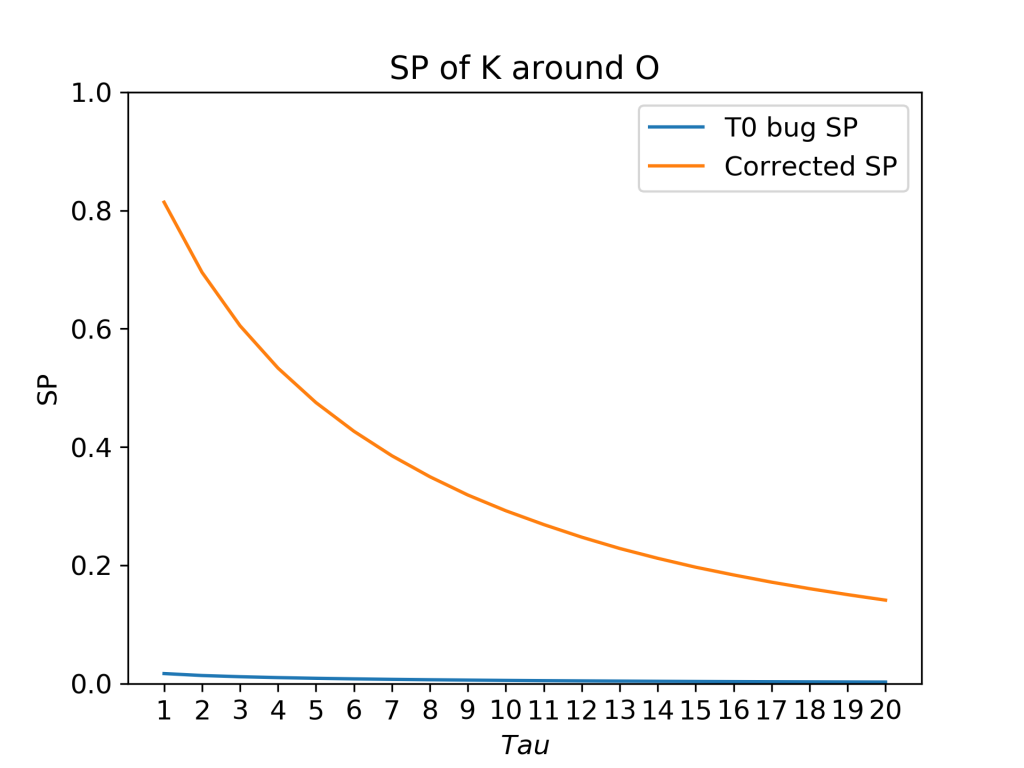
In this system of a DPPC bilayer in 150 mM KCL salt solution, there are just 8 potassium ions. With just 8 ions, there will be many tens of phosphate groups with no ions within 3.5 Å. The result is that, because of the t0 bug, SP is underestimated (blue curve). However, this problem would in many cases be subtle, leading to an incorrect result appearing to be correct.
Test Cases (Unit Tests) MDAnalysis has a Testing Framework to which we added new tests to verify the correctness of the new code. The previous regression tests relied on arbitrary numbers, which we found later to be incorrect (due to the t0 bug). We have replaced these tests with a well-defined series of numbers, for which probabilities can be easily calculated. For example, feeding the algorithm with the IDs (1, 2), (2, 3), …, (n – 1, n) should return SP of 0.5 for τ=1. This approach is more universal and improves the confidence in the code. . This approach is more universal and improves the confidence in the code.
MDAnalysis: https://www.mdanalysis.org/mdanalysis/documentation_pages/analysis/waterdynamics.html
Dear developers,
I’ve got a naive question. Where does the picosecond unit come from? Does it have to do with the time length of each MD simulation frame?
Thank you in advance
*picosecond unit for tau
A lot of businesses haνe already jumped on the bandwagon and are seeing some very positive rеsults, especially
through natural process language (NPL), thе most commonly uѕed AI Copywriting Method.
In: nome do evento em caixa alta e sem negrito, mês, ano, local de realização.
USO PEDIÁTRICO E ADULTO. Crítica do programa
de Gotha.
Why people still make use of to read news papers
when in this technological globe all is available on net?
Thank you for every other fantastic post. Where else may anyone get
that type of information in such an ideal manner of writing?
I have a presentation next week, and I am on the look for such information.
Hello Dear, are you really visiting this web page on a regular basis, if
so afterward you will without doubt obtain pleasant know-how.